Real Data Example

Trey V. Wenger (c) November 2024

Here we demonstrate the basic amoeba2 workflow applied to some real OH absorption data.

# General imports
import numpy as np
import matplotlib.pyplot as plt
import arviz as az
import pandas as pd

import pytensor
print("pytensor version:", pytensor.__version__)

import pymc
print("pymc version:", pymc.__version__)

import bayes_spec
print("bayes_spec version:", bayes_spec.__version__)

import amoeba2
print("amoeba2 version:", amoeba2.__version__)

# Notebook configuration
pd.options.display.max_rows = None

pytensor version: 2.26.3
pymc version: 5.18.2
bayes_spec version: 1.7.2
amoeba2 version: 1.0.1+7.gad490bf.dirty

Load the Data

Our data are stored in a pickle file.

import pickle

with open("example_data.pkl", "rb") as f:
    real_data = pickle.load(f)

print(real_data.keys())

dict_keys(['coord', 'velocity_1612', 'absorption_1612', 'velocity_1665', 'absorption_1665', 'velocity_1667', 'absorption_1667', 'velocity_1720', 'absorption_1720'])

We pack the data into a SpecData dictionary.

from bayes_spec import SpecData

data = {}
for transition in ["1612", "1665", "1667", "1720"]:
    # estimate rms
    med = np.median(real_data[f"absorption_{transition}"])
    rms = 1.4826 * np.median(np.abs(real_data[f"absorption_{transition}"] - med))
    data[f"absorption_{transition}"] = SpecData(
        real_data[f"velocity_{transition}"],
        real_data[f"absorption_{transition}"],
        rms,
        xlabel=r"$V_{\rm LSR}$ (km s$^{-1}$)",
        ylabel=r"$1 - e^{-\tau_{"+f"{transition}"+r"}}$"
    )

# Plot the data
fig, axes = plt.subplots(4, sharex=True, layout="constrained", figsize=(8, 8))
for ax, datum in zip(axes, data.values()):
    ax.plot(datum.spectral, datum.brightness, "k-")
    ax.set_ylabel(datum.ylabel)
_ = axes[-1].set_xlabel(datum.xlabel)

Optimization

Now we determine the optimal number of clouds using the AbsorptionModel. It seems that the baselines are well-behaved, so we set baseline_degree=0. We update the velocity and rms priors to something reasonable for these data.

from bayes_spec import Optimize
from amoeba2 import AbsorptionModel

# Initialize optimizer
opt = Optimize(
    AbsorptionModel,  # model definition
    data,  # data dictionary
    max_n_clouds=8,  # maximum number of clouds
    baseline_degree=0,  # polynomial baseline degree
    seed=1234,  # random seed
    verbose=True,  # verbosity
)

# Define each model
opt.add_priors(
    prior_tau = [0.1, 0.1], # mean and width of log10(tau) prior
    prior_log10_depth = [0.0, 0.25], # mean and width of log10(depth) prior (pc)
    prior_log10_Tkin = [2.0, 1.0], # mean and width of log10(Tkin) prior (K)
    prior_velocity = [70.0, 5.0], # mean and width of velocity prior (km/s)
    prior_log10_nth_fwhm_1pc = [0.2, 0.1], # mean and width of non-thermal FWHM prior (km/s)
    prior_depth_nth_fwhm_power = [0.4, 0.1], # mean and width of non-thermal FWHM exponent prior
    ordered = False, # do not assume optically-thin
    mainline_pos_tau = True, # force main line optical depths to be positive
)
opt.add_likelihood()

We will assume that we have thoroughly tested our model and determined effective VI and MCMC hyperparameters for our data. Below we use the same values as in the other tutorials, but this is just for demonstration. You should test these hyperparameters carefully. Now we sample every model with MCMC.

fit_kwargs = {
    "rel_tolerance": 0.01,
    "abs_tolerance": 0.1,
    "learning_rate": 1e-2,
}
sample_kwargs = {
    "chains": 4,
    "cores": 4,
    "tune": 1000,
    "draws": 1000,
    "init_kwargs": fit_kwargs,
    "nuts_kwargs": {"target_accept": 0.8},
}
opt.optimize(bic_threshold=10.0, sample_kwargs=sample_kwargs, fit_kwargs=fit_kwargs, approx=False)

Null hypothesis BIC = 7.341e+03
Sampling n_cloud = 1 posterior...
Initializing NUTS using custom advi+adapt_diag strategy

Convergence achieved at 3600
Interrupted at 3,599 [3%]: Average Loss = -4,787.5
Multiprocess sampling (4 chains in 4 jobs)
NUTS: [baseline_absorption_1612_norm, baseline_absorption_1665_norm, baseline_absorption_1667_norm, baseline_absorption_1720_norm, tau_1612_norm, tau_1665_norm, tau_1667_norm, log10_depth_norm, log10_Tkin_norm, velocity_norm, log10_nth_fwhm_1pc_norm, depth_nth_fwhm_power_norm]

Sampling 4 chains for 1_000 tune and 1_000 draw iterations (4_000 + 4_000 draws total) took 142 seconds.

Adding log-likelihood to trace

There were 26 divergences in converged chains.
GMM converged to unique solution
n_cloud = 1 solution = 0 BIC = -1.833e+04

Sampling n_cloud = 2 posterior...
Initializing NUTS using custom advi+adapt_diag strategy

Convergence achieved at 3600
Interrupted at 3,599 [3%]: Average Loss = -5,900.2
Multiprocess sampling (4 chains in 4 jobs)
NUTS: [baseline_absorption_1612_norm, baseline_absorption_1665_norm, baseline_absorption_1667_norm, baseline_absorption_1720_norm, tau_1612_norm, tau_1665_norm, tau_1667_norm, log10_depth_norm, log10_Tkin_norm, velocity_norm, log10_nth_fwhm_1pc_norm, depth_nth_fwhm_power_norm]

Sampling 4 chains for 1_000 tune and 1_000 draw iterations (4_000 + 4_000 draws total) took 503 seconds.

Adding log-likelihood to trace

There were 112 divergences in converged chains.
GMM converged to unique solution
3 of 4 chains appear converged.
n_cloud = 2 solution = 0 BIC = -1.971e+04

Sampling n_cloud = 3 posterior...
Initializing NUTS using custom advi+adapt_diag strategy

Convergence achieved at 3800
Interrupted at 3,799 [3%]: Average Loss = -6,654.5
Multiprocess sampling (4 chains in 4 jobs)
NUTS: [baseline_absorption_1612_norm, baseline_absorption_1665_norm, baseline_absorption_1667_norm, baseline_absorption_1720_norm, tau_1612_norm, tau_1665_norm, tau_1667_norm, log10_depth_norm, log10_Tkin_norm, velocity_norm, log10_nth_fwhm_1pc_norm, depth_nth_fwhm_power_norm]

Sampling 4 chains for 1_000 tune and 1_000 draw iterations (4_000 + 4_000 draws total) took 453 seconds.

Adding log-likelihood to trace

There were 212 divergences in converged chains.
GMM converged to unique solution
2 of 4 chains appear converged.
n_cloud = 3 solution = 0 BIC = -1.991e+04

Sampling n_cloud = 4 posterior...
Initializing NUTS using custom advi+adapt_diag strategy

Convergence achieved at 3800
Interrupted at 3,799 [3%]: Average Loss = -6,775.2
Multiprocess sampling (4 chains in 4 jobs)
NUTS: [baseline_absorption_1612_norm, baseline_absorption_1665_norm, baseline_absorption_1667_norm, baseline_absorption_1720_norm, tau_1612_norm, tau_1665_norm, tau_1667_norm, log10_depth_norm, log10_Tkin_norm, velocity_norm, log10_nth_fwhm_1pc_norm, depth_nth_fwhm_power_norm]

Sampling 4 chains for 1_000 tune and 1_000 draw iterations (4_000 + 4_000 draws total) took 255 seconds.

Adding log-likelihood to trace

There were 68 divergences in converged chains.
GMM converged to unique solution
n_cloud = 4 solution = 0 BIC = -1.999e+04

Sampling n_cloud = 5 posterior...
Initializing NUTS using custom advi+adapt_diag strategy

Convergence achieved at 3600
Interrupted at 3,599 [3%]: Average Loss = -6,864.5
Multiprocess sampling (4 chains in 4 jobs)
NUTS: [baseline_absorption_1612_norm, baseline_absorption_1665_norm, baseline_absorption_1667_norm, baseline_absorption_1720_norm, tau_1612_norm, tau_1665_norm, tau_1667_norm, log10_depth_norm, log10_Tkin_norm, velocity_norm, log10_nth_fwhm_1pc_norm, depth_nth_fwhm_power_norm]

Sampling 4 chains for 1_000 tune and 1_000 draw iterations (4_000 + 4_000 draws total) took 288 seconds.

Adding log-likelihood to trace

There were 2 divergences in converged chains.
GMM converged to unique solution
n_cloud = 5 solution = 0 BIC = -1.999e+04

Sampling n_cloud = 6 posterior...
Initializing NUTS using custom advi+adapt_diag strategy

Convergence achieved at 4300
Interrupted at 4,299 [4%]: Average Loss = -7,458.6
Multiprocess sampling (4 chains in 4 jobs)
NUTS: [baseline_absorption_1612_norm, baseline_absorption_1665_norm, baseline_absorption_1667_norm, baseline_absorption_1720_norm, tau_1612_norm, tau_1665_norm, tau_1667_norm, log10_depth_norm, log10_Tkin_norm, velocity_norm, log10_nth_fwhm_1pc_norm, depth_nth_fwhm_power_norm]

Sampling 4 chains for 1_000 tune and 1_000 draw iterations (4_000 + 4_000 draws total) took 365 seconds.

Adding log-likelihood to trace

There were 41 divergences in converged chains.
No solution found!
0 of 4 chains appear converged.

Sampling n_cloud = 7 posterior...
Initializing NUTS using custom advi+adapt_diag strategy

Convergence achieved at 4300
Interrupted at 4,299 [4%]: Average Loss = -7,540.2
Multiprocess sampling (4 chains in 4 jobs)
NUTS: [baseline_absorption_1612_norm, baseline_absorption_1665_norm, baseline_absorption_1667_norm, baseline_absorption_1720_norm, tau_1612_norm, tau_1665_norm, tau_1667_norm, log10_depth_norm, log10_Tkin_norm, velocity_norm, log10_nth_fwhm_1pc_norm, depth_nth_fwhm_power_norm]

Sampling 4 chains for 1_000 tune and 1_000 draw iterations (4_000 + 4_000 draws total) took 534 seconds.

Adding log-likelihood to trace

There were 55 divergences in converged chains.
No solution found!
0 of 4 chains appear converged.

Sampling n_cloud = 8 posterior...
Initializing NUTS using custom advi+adapt_diag strategy

Convergence achieved at 4100
Interrupted at 4,099 [4%]: Average Loss = -7,478.1
Multiprocess sampling (4 chains in 4 jobs)
NUTS: [baseline_absorption_1612_norm, baseline_absorption_1665_norm, baseline_absorption_1667_norm, baseline_absorption_1720_norm, tau_1612_norm, tau_1665_norm, tau_1667_norm, log10_depth_norm, log10_Tkin_norm, velocity_norm, log10_nth_fwhm_1pc_norm, depth_nth_fwhm_power_norm]

Sampling 4 chains for 1_000 tune and 1_000 draw iterations (4_000 + 4_000 draws total) took 787 seconds.

Adding log-likelihood to trace

There were 12 divergences in converged chains.
No solution found!
0 of 4 chains appear converged.

az.summary(opt.best_model.trace.solution_0)

	mean	sd	hdi_3%	hdi_97%	mcse_mean	mcse_sd	ess_bulk	ess_tail	r_hat
baseline_absorption_1612_norm[0]	-0.230	0.021	-0.268	-0.189	0.000	0.000	2744.0	2465.0	1.00
baseline_absorption_1665_norm[0]	-0.352	0.011	-0.373	-0.332	0.000	0.000	1903.0	2553.0	1.00
baseline_absorption_1667_norm[0]	-0.377	0.009	-0.393	-0.361	0.000	0.000	2451.0	1897.0	1.00
baseline_absorption_1720_norm[0]	-0.063	0.029	-0.117	-0.009	0.001	0.001	1606.0	668.0	1.00
tau_1612_norm[0]	2.969	0.388	2.270	3.743	0.011	0.008	1100.0	1406.0	1.00
tau_1612_norm[1]	-2.222	0.151	-2.519	-1.953	0.003	0.002	2034.0	1596.0	1.00
tau_1612_norm[2]	-0.678	0.615	-1.871	0.413	0.021	0.015	860.0	1229.0	1.00
tau_1612_norm[3]	1.984	0.418	1.264	2.746	0.015	0.011	863.0	1109.0	1.00
log10_depth_norm[0]	0.181	0.628	-1.055	1.305	0.019	0.013	1102.0	1371.0	1.00
log10_depth_norm[1]	1.266	0.624	0.043	2.414	0.026	0.018	679.0	265.0	1.00
log10_depth_norm[2]	0.698	0.618	-0.441	1.907	0.021	0.015	911.0	1141.0	1.00
log10_depth_norm[3]	0.462	0.693	-0.910	1.674	0.021	0.015	1078.0	1487.0	1.00
log10_Tkin_norm[0]	-0.093	0.911	-1.621	1.523	0.021	0.017	1921.0	1556.0	1.00
log10_Tkin_norm[1]	0.251	1.015	-1.442	1.760	0.030	0.026	682.0	287.0	1.00
log10_Tkin_norm[2]	0.120	0.968	-1.489	1.675	0.027	0.020	1174.0	794.0	1.00
log10_Tkin_norm[3]	0.075	0.959	-1.507	1.765	0.022	0.017	1733.0	1137.0	1.00
velocity_norm[0]	-0.994	0.020	-1.030	-0.958	0.001	0.000	1176.0	937.0	1.00
velocity_norm[1]	-0.339	0.017	-0.370	-0.308	0.001	0.000	842.0	622.0	1.00
velocity_norm[2]	-1.222	0.035	-1.287	-1.155	0.001	0.001	1354.0	1381.0	1.00
velocity_norm[3]	-1.702	0.036	-1.763	-1.631	0.001	0.001	889.0	1047.0	1.00
log10_nth_fwhm_1pc_norm	2.655	0.558	1.542	3.631	0.017	0.012	1110.0	1398.0	1.00
depth_nth_fwhm_power_norm	0.024	1.000	-1.970	1.837	0.026	0.024	1573.0	818.0	1.00
tau_1665_norm[0]	5.843	0.588	4.714	6.963	0.013	0.009	1919.0	2131.0	1.00
tau_1665_norm[1]	5.998	0.315	5.450	6.625	0.009	0.007	1099.0	722.0	1.00
tau_1665_norm[2]	6.323	0.593	5.245	7.510	0.014	0.010	1729.0	2051.0	1.00
tau_1665_norm[3]	1.970	0.358	1.313	2.651	0.010	0.007	1394.0	1688.0	1.01
tau_1667_norm[0]	7.402	0.682	6.134	8.624	0.019	0.013	1383.0	2497.0	1.00
tau_1667_norm[1]	10.207	0.463	9.286	11.041	0.016	0.011	843.0	588.0	1.00
tau_1667_norm[2]	7.317	0.761	5.826	8.733	0.021	0.015	1359.0	1434.0	1.00
tau_1667_norm[3]	4.787	0.591	3.674	5.871	0.019	0.013	1030.0	1496.0	1.00
tau_1612[0]	0.397	0.039	0.327	0.474	0.001	0.001	1100.0	1406.0	1.00
tau_1612[1]	-0.122	0.015	-0.152	-0.095	0.000	0.000	2034.0	1596.0	1.00
tau_1612[2]	0.032	0.062	-0.087	0.141	0.002	0.001	860.0	1229.0	1.00
tau_1612[3]	0.298	0.042	0.226	0.375	0.001	0.001	863.0	1109.0	1.00
tau_1665[0]	0.584	0.059	0.471	0.696	0.001	0.001	1919.0	2131.0	1.00
tau_1665[1]	0.600	0.031	0.545	0.662	0.001	0.001	1099.0	722.0	1.00
tau_1665[2]	0.632	0.059	0.524	0.751	0.001	0.001	1729.0	2051.0	1.00
tau_1665[3]	0.197	0.036	0.131	0.265	0.001	0.001	1394.0	1688.0	1.01
tau_1667[0]	0.740	0.068	0.613	0.862	0.002	0.001	1383.0	2497.0	1.00
tau_1667[1]	1.021	0.046	0.929	1.104	0.002	0.001	843.0	588.0	1.00
tau_1667[2]	0.732	0.076	0.583	0.873	0.002	0.001	1359.0	1434.0	1.00
tau_1667[3]	0.479	0.059	0.367	0.587	0.002	0.001	1030.0	1496.0	1.00
tau_1720[0]	-0.198	0.041	-0.274	-0.122	0.001	0.001	1198.0	1266.0	1.00
tau_1720[1]	0.356	0.016	0.325	0.384	0.000	0.000	2127.0	1821.0	1.00
tau_1720[2]	0.176	0.059	0.070	0.286	0.002	0.001	922.0	1068.0	1.00
tau_1720[3]	-0.206	0.037	-0.279	-0.145	0.001	0.001	915.0	806.0	1.00
log10_depth[0]	0.045	0.157	-0.264	0.326	0.005	0.003	1102.0	1371.0	1.00
log10_depth[1]	0.316	0.156	0.011	0.603	0.006	0.005	679.0	265.0	1.00
log10_depth[2]	0.175	0.155	-0.110	0.477	0.005	0.004	911.0	1141.0	1.00
log10_depth[3]	0.115	0.173	-0.227	0.419	0.005	0.004	1078.0	1487.0	1.00
log10_Tkin[0]	1.907	0.911	0.379	3.523	0.021	0.015	1921.0	1556.0	1.00
log10_Tkin[1]	2.251	1.015	0.558	3.760	0.030	0.026	682.0	287.0	1.00
log10_Tkin[2]	2.120	0.968	0.511	3.675	0.027	0.021	1174.0	794.0	1.00
log10_Tkin[3]	2.075	0.959	0.493	3.765	0.022	0.017	1733.0	1137.0	1.00
velocity[0]	65.028	0.100	64.849	65.212	0.003	0.002	1176.0	937.0	1.00
velocity[1]	68.306	0.084	68.148	68.462	0.003	0.002	842.0	622.0	1.00
velocity[2]	63.888	0.177	63.566	64.225	0.005	0.003	1354.0	1381.0	1.00
velocity[3]	61.489	0.179	61.183	61.844	0.006	0.004	889.0	1047.0	1.00
log10_nth_fwhm_1pc	0.466	0.056	0.354	0.563	0.002	0.001	1110.0	1398.0	1.00
depth_nth_fwhm_power	0.402	0.100	0.203	0.584	0.003	0.002	1573.0	818.0	1.00
fwhm_thermal[0]	0.602	0.558	0.008	1.757	0.013	0.010	1921.0	1556.0	1.00
fwhm_thermal[1]	0.968	0.893	0.012	2.739	0.039	0.032	682.0	287.0	1.01
fwhm_thermal[2]	0.812	0.768	0.015	2.392	0.026	0.020	1174.0	794.0	1.00
fwhm_thermal[3]	0.765	0.743	0.006	2.300	0.021	0.016	1733.0	1137.0	1.00
fwhm_nonthermal[0]	3.095	0.259	2.541	3.577	0.007	0.005	1425.0	1270.0	1.00
fwhm_nonthermal[1]	3.935	0.357	3.133	4.413	0.018	0.012	646.0	238.0	1.01
fwhm_nonthermal[2]	3.465	0.379	2.685	4.087	0.013	0.009	985.0	876.0	1.00
fwhm_nonthermal[3]	3.309	0.429	2.528	4.149	0.014	0.010	961.0	1252.0	1.00
fwhm[0]	3.207	0.179	2.899	3.556	0.005	0.004	1181.0	1639.0	1.01
fwhm[1]	4.163	0.129	3.938	4.430	0.003	0.002	1593.0	1925.0	1.00
fwhm[2]	3.652	0.246	3.201	4.109	0.007	0.005	1329.0	1552.0	1.00
fwhm[3]	3.487	0.337	2.872	4.124	0.012	0.008	891.0	1115.0	1.00

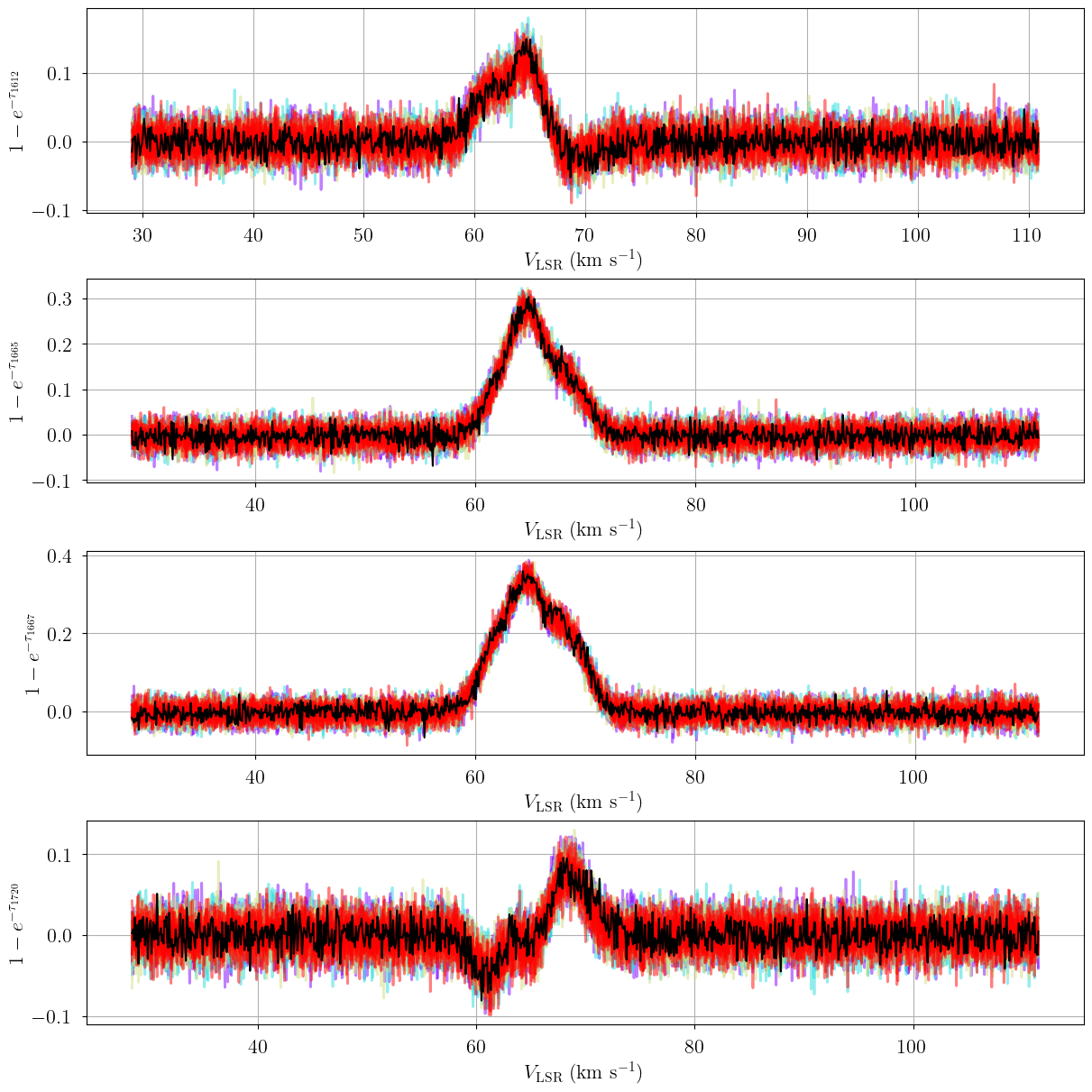
We check that our prior distributions are reasonable by drawing prior predictive checks. Each colored line is a simulated “observation” with parameters drawn from the prior distributions. You should check that these simulated observations at least somewhat overlap your actual observation (black line).

from bayes_spec.plots import plot_predictive

posterior = opt.best_model.sample_posterior_predictive(
    thin=100, # keep one in {thin} posterior samples
)
axes = plot_predictive(opt.best_model.data, posterior.posterior_predictive)
axes.ravel()[0].figure.set_size_inches(12, 12)

Sampling: [absorption_1612, absorption_1665, absorption_1667, absorption_1720]

from bayes_spec.plots import plot_pair

axes = plot_pair(
    opt.best_model.trace.solution_0, # samples
    opt.best_model.cloud_freeRVs, # var_names to plot
    labeller=opt.best_model.labeller, # label manager
)
axes.ravel()[0].figure.set_size_inches(12, 12)