AbsorptionModel Tutorial

Trey V. Wenger (c) November 2024

Here we demonstrate the basic features of the AbsorptionModel model. AbsorptionModel models the 1612, 1665, 1667, and 1720 MHz hyperfine transitions of OH and predicts their absorption spectra: \(1-\exp(-\tau)\).

# General imports
import numpy as np
import matplotlib.pyplot as plt
import arviz as az
import pandas as pd

import pytensor
print("pytensor version:", pytensor.__version__)

import pymc
print("pymc version:", pymc.__version__)

import bayes_spec
print("bayes_spec version:", bayes_spec.__version__)

import amoeba2
print("amoeba2 version:", amoeba2.__version__)

# Notebook configuration
pd.options.display.max_rows = None

pytensor version: 2.26.3
pymc version: 5.18.2
bayes_spec version: 1.7.2
amoeba2 version: 1.0.1+7.gad490bf.dirty

Simulating Data

To test the model, we must simulate some data. We can do this with AbsorptionModel, but we must pack a “dummy” data structure first. The model expects the observations to be named "absorption_1612", "absorption_1665", "absorption_1667", and "absorption_1720".

from bayes_spec import SpecData

# spectral axes definition
velo_axis = {
    "1612": np.linspace(-20.0, 20.0, 400), # km s-1
    "1665": np.linspace(-18.0, 18.0, 450),
    "1667": np.linspace(-18.0, 18.0, 450),
    "1720": np.linspace(-15.0, 15.0, 500),
}

# data noise can either be a scalar (assumed constant noise across the spectrum)
# or an array of the same length as the data
rms_absorption = {
    "1612": 0.01,
    "1665": 0.01,
    "1667": 0.01,
    "1720": 0.01,
}

# spectral data. In this case, we just throw in some random data for now
# since we are only doing this in order to simulate some actual data.
absorption = {label: rms_absorption[label] * np.random.randn(len(velo_axis[label])) for label in velo_axis.keys()}

# TauModel expects four observations
dummy_data = {
    f"absorption_{label}": SpecData(
        velo_axis[label],
        absorption[label],
        rms_absorption[label],
        xlabel=r"$V_{\rm LSR}$ (km s$^{-1}$)",
        ylabel=r"$1 - e^{-\tau_{"+f"{label}"+r"}}$"
    )
    for label in velo_axis.keys()
}

# Plot dummy data
fig, axes = plt.subplots(4, sharex=True, layout="constrained", figsize=(8, 8))
for ax, dummy_datum in zip(axes, dummy_data.values()):
    ax.plot(dummy_datum.spectral, dummy_datum.brightness, "k-")
    ax.set_ylabel(dummy_datum.ylabel)
_ = axes[-1].set_xlabel(dummy_datum.xlabel)

Now that we have a dummy data format, we can generate a simulated observation by evaluating the likelihood.

from amoeba2 import AbsorptionModel

# Initialize and define the model
n_clouds = 3
baseline_degree = 0
model = AbsorptionModel(
    dummy_data,
    n_clouds=n_clouds,
    baseline_degree=baseline_degree,
    seed=1234,
    verbose=True
)
model.add_priors(
    prior_tau = [0.1, 0.1], # mean and width of log10(tau) prior
    prior_log10_depth = [0.0, 0.25], # mean and width of log10(depth) prior (pc)
    prior_log10_Tkin = [2.0, 1.0], # mean and width of log10(Tkin) prior (K)
    prior_velocity = [0.0, 5.0], # mean and width of velocity prior (km/s)
    prior_log10_nth_fwhm_1pc = [0.2, 0.1], # mean and width of non-thermal FWHM prior (km/s)
    prior_depth_nth_fwhm_power = [0.4, 0.1], # mean and width of non-thermal FWHM exponent prior
    ordered = False, # do not assume optically-thin
    mainline_pos_tau = True, # force main line optical depths to be positive
)
model.add_likelihood()

# Evaluate likelihood for given model parameters
sim_params = {
    "tau_1612": np.array([-0.05, 0.05, 0.05]),
    "tau_1665": np.array([0.05, 0.1, 0.02]),
    "tau_1667": np.array([0.02, 0.02, 0.1]),
    "log10_depth": np.array([0.0, 0.25, -0.25]),
    "log10_Tkin": np.array([1.25, 1.75, 1.0]),
    "velocity": np.array([-3.0, 1.0, 3.0]),
    "log10_nth_fwhm_1pc": 0.2,
    "depth_nth_fwhm_power": 0.3,
    "baseline_absorption_1612_norm": [0.0],
    "baseline_absorption_1665_norm": [0.0],
    "baseline_absorption_1667_norm": [0.0],
    "baseline_absorption_1720_norm": [0.0],
}

data = {}
for i, label in enumerate(velo_axis.keys()):
    sim_absorption = model.model[f"absorption_{label}"].eval(sim_params, on_unused_input="ignore")
    data[f"absorption_{label}"] = SpecData(
        velo_axis[label],
        sim_absorption,
        rms_absorption[label],
        xlabel=r"$V_{\rm LSR}$ (km s$^{-1}$)",
        ylabel=r"$1 - e^{-\tau_{"+f"{label}"+r"}}$"
    )

# Plot data
fig, axes = plt.subplots(4, sharex=True, layout="constrained", figsize=(8, 8))
for ax, datum in zip(axes, data.values()):
    ax.plot(datum.spectral, datum.brightness, "k-")
    ax.set_ylabel(datum.ylabel)
_ = axes[-1].set_xlabel(datum.xlabel)

Model Definition

Finally, with our model definition and (simulated) data in hand, we can explore the capabilities of TauModel. Here we create a new model with the simulated data.

# Initialize and define the model
model = AbsorptionModel(
    data,
    n_clouds=n_clouds,
    baseline_degree=baseline_degree,
    seed=1234,
    verbose=True
)
model.add_priors(
    prior_tau = [0.1, 0.1], # mean and width of log10(tau) prior
    prior_log10_depth = [0.0, 0.25], # mean and width of log10(depth) prior (pc)
    prior_log10_Tkin = [2.0, 1.0], # mean and width of log10(Tkin) prior (K)
    prior_velocity = [0.0, 5.0], # mean and width of velocity prior (km/s)
    prior_log10_nth_fwhm_1pc = [0.2, 0.1], # mean and width of non-thermal FWHM prior (km/s)
    prior_depth_nth_fwhm_power = [0.4, 0.1], # mean and width of non-thermal FWHM exponent prior
    ordered = False, # do not assume optically-thin
    mainline_pos_tau = True, # force main line optical depths to be positive
)
model.add_likelihood()

# Plot model graph
gviz = pymc.model_to_graphviz(model.model)
gviz.graph_attr["rankdir"] = "TB"
gviz.graph_attr["splines"] = "ortho"
# gviz.graph_attr["newrank"] = "true"
gviz.graph_attr["rank"] = "same"
gviz.graph_attr["ranksep"] = "1.0"
gviz.graph_attr["nodesep"] = "0.3"
gviz.render('absorption_model', format='png')
gviz

# model string representation
print(model.model.str_repr())

baseline_absorption_1612_norm ~ Normal(0, 1)
baseline_absorption_1665_norm ~ Normal(0, 1)
baseline_absorption_1667_norm ~ Normal(0, 1)
baseline_absorption_1720_norm ~ Normal(0, 1)
                tau_1612_norm ~ Normal(0, 1)
                tau_1665_norm ~ HalfNormal(0, 1)
                tau_1667_norm ~ HalfNormal(0, 1)
             log10_depth_norm ~ Normal(0, 1)
              log10_Tkin_norm ~ Normal(0, 1)
                velocity_norm ~ Normal(0, 1)
      log10_nth_fwhm_1pc_norm ~ Normal(0, 1)
    depth_nth_fwhm_power_norm ~ Normal(0, 1)
                     tau_1612 ~ Deterministic(f(tau_1612_norm))
                     tau_1665 ~ Deterministic(f(tau_1665_norm))
                     tau_1667 ~ Deterministic(f(tau_1667_norm))
                     tau_1720 ~ Deterministic(f(tau_1612_norm, tau_1667_norm, tau_1665_norm))
                  log10_depth ~ Deterministic(f(log10_depth_norm))
                   log10_Tkin ~ Deterministic(f(log10_Tkin_norm))
                     velocity ~ Deterministic(f(velocity_norm))
           log10_nth_fwhm_1pc ~ Deterministic(f(log10_nth_fwhm_1pc_norm))
         depth_nth_fwhm_power ~ Deterministic(f(depth_nth_fwhm_power_norm))
                 fwhm_thermal ~ Deterministic(f(log10_Tkin_norm))
              fwhm_nonthermal ~ Deterministic(f(depth_nth_fwhm_power_norm, log10_depth_norm, log10_nth_fwhm_1pc_norm))
                         fwhm ~ Deterministic(f(depth_nth_fwhm_power_norm, log10_depth_norm, log10_nth_fwhm_1pc_norm, log10_Tkin_norm))
              absorption_1612 ~ Normal(f(baseline_absorption_1612_norm, tau_1612_norm, velocity_norm, depth_nth_fwhm_power_norm, log10_depth_norm, log10_nth_fwhm_1pc_norm, log10_Tkin_norm), <constant>)
              absorption_1665 ~ Normal(f(tau_1665_norm, baseline_absorption_1665_norm, velocity_norm, depth_nth_fwhm_power_norm, log10_depth_norm, log10_nth_fwhm_1pc_norm, log10_Tkin_norm), <constant>)
              absorption_1667 ~ Normal(f(tau_1667_norm, baseline_absorption_1667_norm, velocity_norm, depth_nth_fwhm_power_norm, log10_depth_norm, log10_nth_fwhm_1pc_norm, log10_Tkin_norm), <constant>)
              absorption_1720 ~ Normal(f(baseline_absorption_1720_norm, tau_1612_norm, tau_1667_norm, tau_1665_norm, velocity_norm, depth_nth_fwhm_power_norm, log10_depth_norm, log10_nth_fwhm_1pc_norm, log10_Tkin_norm), <constant>)

We check that our prior distributions are reasonable by drawing prior predictive checks. Each colored line is a simulated “observation” with parameters drawn from the prior distributions. You should check that these simulated observations at least somewhat overlap your actual observation (black line).

from bayes_spec.plots import plot_predictive

# prior predictive check
prior = model.sample_prior_predictive(
    samples=100,  # prior predictive samples
)
axes = plot_predictive(model.data, prior.prior_predictive)
axes.ravel()[0].figure.set_size_inches(12, 12)

Sampling: [absorption_1612, absorption_1665, absorption_1667, absorption_1720, baseline_absorption_1612_norm, baseline_absorption_1665_norm, baseline_absorption_1667_norm, baseline_absorption_1720_norm, depth_nth_fwhm_power_norm, log10_Tkin_norm, log10_depth_norm, log10_nth_fwhm_1pc_norm, tau_1612_norm, tau_1665_norm, tau_1667_norm, velocity_norm]

We can also investigate the effect of our chosen priors on the deterministic quantities.

from bayes_spec.plots import plot_pair

var_names = ["fwhm_thermal", "log10_Tkin", "fwhm_nonthermal", "log10_depth"]
_ = plot_pair(
    prior.prior, # samples
    var_names, # var_names to plot
    labeller=model.labeller, # label manager
)

Variational Inference

We can approximate the posterior distribution using variational inference.

import time

start = time.time()
model.fit(
    n = 100_000, # maximum number of VI iterations
    draws = 1_000, # number of posterior samples
    rel_tolerance = 0.01, # VI relative convergence threshold
    abs_tolerance = 0.1, # VI absolute convergence threshold
    learning_rate = 1e-2, # VI learning rate
)
end = time.time()
print(f"Runtime: {(end-start)/60.0:.2f} minutes")

Convergence achieved at 3300
Interrupted at 3,299 [3%]: Average Loss = -4,984.2

Runtime: 0.30 minutes

az.summary(model.trace.posterior)

arviz - WARNING - Shape validation failed: input_shape: (1, 1000), minimum_shape: (chains=2, draws=4)

	mean	sd	hdi_3%	hdi_97%	mcse_mean	mcse_sd	ess_bulk	ess_tail	r_hat
baseline_absorption_1612_norm[0]	-0.087	0.041	-0.168	-0.011	0.001	0.001	979.0	1025.0	NaN
baseline_absorption_1665_norm[0]	-0.302	0.034	-0.363	-0.238	0.001	0.001	930.0	777.0	NaN
baseline_absorption_1667_norm[0]	-0.252	0.033	-0.313	-0.194	0.001	0.001	1025.0	995.0	NaN
baseline_absorption_1720_norm[0]	0.008	0.040	-0.065	0.082	0.001	0.001	1090.0	1002.0	NaN
tau_1612_norm[0]	-0.538	0.036	-0.599	-0.467	0.001	0.001	967.0	901.0	NaN
tau_1612_norm[1]	-1.467	0.034	-1.525	-1.397	0.001	0.001	921.0	971.0	NaN
tau_1612_norm[2]	-0.473	0.031	-0.534	-0.419	0.001	0.001	1007.0	1026.0	NaN
log10_depth_norm[0]	0.597	0.266	0.120	1.121	0.008	0.006	1047.0	937.0	NaN
log10_depth_norm[1]	-0.207	0.311	-0.759	0.370	0.010	0.008	917.0	822.0	NaN
log10_depth_norm[2]	-0.801	0.230	-1.238	-0.379	0.007	0.005	1087.0	937.0	NaN
log10_Tkin_norm[0]	-0.297	0.666	-1.574	0.901	0.022	0.015	961.0	996.0	NaN
log10_Tkin_norm[1]	-0.549	0.645	-1.697	0.691	0.019	0.015	1105.0	982.0	NaN
log10_Tkin_norm[2]	-0.630	0.685	-2.041	0.532	0.023	0.016	870.0	843.0	NaN
velocity_norm[0]	0.203	0.010	0.184	0.222	0.000	0.000	831.0	979.0	NaN
velocity_norm[1]	-0.604	0.011	-0.626	-0.585	0.000	0.000	977.0	1026.0	NaN
velocity_norm[2]	0.616	0.007	0.603	0.630	0.000	0.000	1108.0	919.0	NaN
log10_nth_fwhm_1pc_norm	-0.162	0.149	-0.461	0.086	0.005	0.003	1070.0	982.0	NaN
depth_nth_fwhm_power_norm	-0.569	0.734	-2.139	0.641	0.024	0.017	962.0	983.0	NaN
tau_1665_norm[0]	1.026	0.051	0.940	1.126	0.002	0.001	608.0	952.0	NaN
tau_1665_norm[1]	0.450	0.046	0.359	0.529	0.002	0.001	916.0	916.0	NaN
tau_1665_norm[2]	0.219	0.045	0.146	0.308	0.002	0.001	923.0	1023.0	NaN
tau_1667_norm[0]	0.220	0.055	0.123	0.318	0.002	0.001	946.0	988.0	NaN
tau_1667_norm[1]	0.227	0.048	0.148	0.323	0.002	0.001	960.0	802.0	NaN
tau_1667_norm[2]	1.036	0.048	0.941	1.126	0.002	0.001	970.0	955.0	NaN
tau_1612[0]	0.046	0.004	0.040	0.053	0.000	0.000	967.0	901.0	NaN
tau_1612[1]	-0.047	0.003	-0.052	-0.040	0.000	0.000	921.0	971.0	NaN
tau_1612[2]	0.053	0.003	0.047	0.058	0.000	0.000	1007.0	1026.0	NaN
tau_1665[0]	0.103	0.005	0.094	0.113	0.000	0.000	608.0	952.0	NaN
tau_1665[1]	0.045	0.005	0.036	0.053	0.000	0.000	916.0	916.0	NaN
tau_1665[2]	0.022	0.005	0.015	0.031	0.000	0.000	923.0	1023.0	NaN
tau_1667[0]	0.022	0.005	0.012	0.032	0.000	0.000	946.0	988.0	NaN
tau_1667[1]	0.023	0.005	0.015	0.032	0.000	0.000	960.0	802.0	NaN
tau_1667[2]	0.104	0.005	0.094	0.113	0.000	0.000	970.0	955.0	NaN
tau_1720[0]	-0.023	0.004	-0.030	-0.016	0.000	0.000	916.0	1023.0	NaN
tau_1720[1]	0.058	0.004	0.051	0.064	0.000	0.000	924.0	975.0	NaN
tau_1720[2]	-0.037	0.003	-0.043	-0.031	0.000	0.000	965.0	953.0	NaN
log10_depth[0]	0.149	0.066	0.030	0.280	0.002	0.001	1047.0	937.0	NaN
log10_depth[1]	-0.052	0.078	-0.190	0.093	0.003	0.002	917.0	822.0	NaN
log10_depth[2]	-0.200	0.058	-0.310	-0.095	0.002	0.001	1087.0	937.0	NaN
log10_Tkin[0]	1.703	0.666	0.426	2.901	0.022	0.015	961.0	996.0	NaN
log10_Tkin[1]	1.451	0.645	0.303	2.691	0.019	0.014	1105.0	982.0	NaN
log10_Tkin[2]	1.370	0.685	-0.041	2.532	0.023	0.016	870.0	843.0	NaN
velocity[0]	1.017	0.051	0.922	1.111	0.002	0.001	831.0	979.0	NaN
velocity[1]	-3.022	0.056	-3.131	-2.923	0.002	0.001	977.0	1026.0	NaN
velocity[2]	3.079	0.036	3.013	3.148	0.001	0.001	1108.0	919.0	NaN
log10_nth_fwhm_1pc	0.184	0.015	0.154	0.209	0.000	0.000	1070.0	982.0	NaN
depth_nth_fwhm_power	0.343	0.073	0.186	0.464	0.002	0.002	962.0	983.0	NaN
fwhm_thermal[0]	0.401	0.354	0.035	1.021	0.012	0.008	961.0	996.0	NaN
fwhm_thermal[1]	0.293	0.250	0.017	0.704	0.007	0.005	1105.0	982.0	NaN
fwhm_thermal[2]	0.281	0.304	0.013	0.630	0.010	0.007	870.0	843.0	NaN
fwhm_nonthermal[0]	1.722	0.118	1.514	1.954	0.004	0.003	919.0	851.0	NaN
fwhm_nonthermal[1]	1.470	0.103	1.298	1.677	0.003	0.002	908.0	729.0	NaN
fwhm_nonthermal[2]	1.306	0.083	1.139	1.451	0.003	0.002	1081.0	881.0	NaN
fwhm[0]	1.796	0.192	1.522	2.121	0.006	0.004	945.0	926.0	NaN
fwhm[1]	1.516	0.145	1.301	1.748	0.004	0.003	1044.0	942.0	NaN
fwhm[2]	1.359	0.190	1.147	1.548	0.006	0.004	1027.0	908.0	NaN

posterior = model.sample_posterior_predictive(
    thin=100, # keep one in {thin} posterior samples
)
axes = plot_predictive(model.data, posterior.posterior_predictive)
axes.ravel()[0].figure.set_size_inches(12, 12)

Sampling: [absorption_1612, absorption_1665, absorption_1667, absorption_1720]

Posterior Sampling: MCMC

We can sample from the posterior distribution using MCMC.

start = time.time()
model.sample(
    init = "advi+adapt_diag", # initialization strategy
    tune = 1000, # tuning samples
    draws = 1000, # posterior samples
    chains = 4, # number of independent chains
    cores = 4, # number of parallel chains
    init_kwargs = {"rel_tolerance": 0.01, "abs_tolerance": 0.1, "learning_rate": 1e-2}, # VI initialization arguments
    nuts_kwargs = {"target_accept": 0.8}, # NUTS arguments
)
end = time.time()
print(f"Runtime: {(end-start)/60.0:.2f} minutes")

Initializing NUTS using custom advi+adapt_diag strategy

Convergence achieved at 3300
Interrupted at 3,299 [3%]: Average Loss = -4,984.2
Multiprocess sampling (4 chains in 4 jobs)
NUTS: [baseline_absorption_1612_norm, baseline_absorption_1665_norm, baseline_absorption_1667_norm, baseline_absorption_1720_norm, tau_1612_norm, tau_1665_norm, tau_1667_norm, log10_depth_norm, log10_Tkin_norm, velocity_norm, log10_nth_fwhm_1pc_norm, depth_nth_fwhm_power_norm]

Sampling 4 chains for 1_000 tune and 1_000 draw iterations (4_000 + 4_000 draws total) took 51 seconds.

Adding log-likelihood to trace

There were 1 divergences in converged chains.
Runtime: 1.37 minutes

model.solve(kl_div_threshold=0.1)

GMM converged to unique solution

Check that the effective sample sizes are large and the covergence statistic r_hat is close to 1! If not, you may have to increase the number of tuning steps (tune=2000) or the NUTS acceptance rate (target_accept=0.9).

print("solutions:", model.solutions)
az.summary(model.trace["solution_0"])
# this also works: az.summary(model.trace.solution_0)

solutions: [0]

	mean	sd	hdi_3%	hdi_97%	mcse_mean	mcse_sd	ess_bulk	ess_tail	r_hat
baseline_absorption_1612_norm[0]	-0.092	0.041	-0.173	-0.017	0.002	0.001	676.0	142.0	1.01
baseline_absorption_1665_norm[0]	-0.311	0.035	-0.376	-0.244	0.001	0.000	3064.0	2608.0	1.00
baseline_absorption_1667_norm[0]	-0.250	0.034	-0.321	-0.189	0.001	0.000	2473.0	1527.0	1.00
baseline_absorption_1720_norm[0]	0.009	0.035	-0.054	0.080	0.001	0.001	3761.0	2457.0	1.00
tau_1612_norm[0]	-0.537	0.039	-0.607	-0.464	0.001	0.001	2110.0	1863.0	1.00
tau_1612_norm[1]	-1.456	0.035	-1.521	-1.393	0.001	0.001	1252.0	2315.0	1.00
tau_1612_norm[2]	-0.486	0.036	-0.548	-0.418	0.001	0.001	1576.0	945.0	1.00
log10_depth_norm[0]	0.478	0.773	-1.010	1.966	0.035	0.025	560.0	263.0	1.01
log10_depth_norm[1]	-0.165	0.662	-1.428	1.066	0.020	0.014	1043.0	1320.0	1.00
log10_depth_norm[2]	-0.648	0.626	-1.806	0.479	0.019	0.013	1108.0	1827.0	1.00
log10_Tkin_norm[0]	0.096	0.817	-1.381	1.286	0.035	0.025	188.0	47.0	1.02
log10_Tkin_norm[1]	-0.305	0.777	-1.705	0.891	0.025	0.017	699.0	693.0	1.00
log10_Tkin_norm[2]	-0.443	0.719	-1.740	0.713	0.026	0.018	421.0	231.0	1.01
velocity_norm[0]	0.205	0.010	0.187	0.223	0.000	0.000	1709.0	1777.0	1.00
velocity_norm[1]	-0.607	0.008	-0.623	-0.592	0.000	0.000	1232.0	1149.0	1.00
velocity_norm[2]	0.611	0.006	0.600	0.621	0.000	0.000	2211.0	2861.0	1.00
log10_nth_fwhm_1pc_norm	-0.449	0.607	-1.678	0.652	0.043	0.052	254.0	54.0	1.02
depth_nth_fwhm_power_norm	-0.135	1.001	-2.066	1.640	0.045	0.032	500.0	218.0	1.00
tau_1665_norm[0]	1.038	0.064	0.914	1.154	0.001	0.001	2110.0	2591.0	1.00
tau_1665_norm[1]	0.441	0.047	0.355	0.528	0.001	0.001	1530.0	1714.0	1.00
tau_1665_norm[2]	0.212	0.048	0.128	0.305	0.002	0.001	855.0	1050.0	1.01
tau_1667_norm[0]	0.221	0.054	0.111	0.317	0.002	0.001	1151.0	1352.0	1.01
tau_1667_norm[1]	0.217	0.046	0.134	0.303	0.001	0.001	919.0	984.0	1.00
tau_1667_norm[2]	1.016	0.055	0.912	1.117	0.002	0.002	540.0	358.0	1.01
tau_1612[0]	0.046	0.004	0.039	0.054	0.000	0.000	2110.0	1863.0	1.00
tau_1612[1]	-0.046	0.003	-0.052	-0.039	0.000	0.000	1252.0	2315.0	1.00
tau_1612[2]	0.051	0.004	0.045	0.058	0.000	0.000	1576.0	945.0	1.00
tau_1665[0]	0.104	0.006	0.091	0.115	0.000	0.000	2110.0	2591.0	1.00
tau_1665[1]	0.044	0.005	0.035	0.053	0.000	0.000	1530.0	1714.0	1.00
tau_1665[2]	0.021	0.005	0.013	0.031	0.000	0.000	855.0	1050.0	1.01
tau_1667[0]	0.022	0.005	0.011	0.032	0.000	0.000	1151.0	1352.0	1.01
tau_1667[1]	0.022	0.005	0.013	0.030	0.000	0.000	919.0	984.0	1.00
tau_1667[2]	0.102	0.006	0.091	0.112	0.000	0.000	540.0	358.0	1.01
tau_1720[0]	-0.023	0.004	-0.029	-0.017	0.000	0.000	2231.0	1364.0	1.01
tau_1720[1]	0.057	0.004	0.050	0.064	0.000	0.000	923.0	1877.0	1.01
tau_1720[2]	-0.036	0.003	-0.042	-0.031	0.000	0.000	2450.0	2395.0	1.00
log10_depth[0]	0.120	0.193	-0.253	0.491	0.009	0.006	560.0	263.0	1.01
log10_depth[1]	-0.041	0.166	-0.357	0.267	0.005	0.004	1043.0	1320.0	1.00
log10_depth[2]	-0.162	0.157	-0.451	0.120	0.005	0.003	1108.0	1827.0	1.00
log10_Tkin[0]	2.096	0.817	0.619	3.286	0.035	0.032	188.0	47.0	1.02
log10_Tkin[1]	1.695	0.777	0.295	2.891	0.025	0.022	699.0	693.0	1.00
log10_Tkin[2]	1.557	0.719	0.260	2.713	0.026	0.027	421.0	231.0	1.01
velocity[0]	1.026	0.049	0.934	1.117	0.001	0.001	1709.0	1777.0	1.00
velocity[1]	-3.033	0.042	-3.117	-2.959	0.001	0.001	1232.0	1149.0	1.00
velocity[2]	3.055	0.028	2.999	3.105	0.001	0.000	2211.0	2861.0	1.00
log10_nth_fwhm_1pc	0.155	0.061	0.032	0.265	0.004	0.003	254.0	54.0	1.02
depth_nth_fwhm_power	0.386	0.100	0.193	0.564	0.004	0.004	500.0	218.0	1.00
fwhm_thermal[0]	0.664	0.473	0.020	1.496	0.035	0.036	188.0	47.0	1.02
fwhm_thermal[1]	0.409	0.298	0.023	0.990	0.013	0.010	699.0	693.0	1.00
fwhm_thermal[2]	0.336	0.234	0.021	0.794	0.014	0.012	421.0	231.0	1.01
fwhm_nonthermal[0]	1.602	0.265	1.008	2.004	0.025	0.018	219.0	41.0	1.02
fwhm_nonthermal[1]	1.387	0.158	1.078	1.654	0.010	0.007	355.0	306.0	1.01
fwhm_nonthermal[2]	1.249	0.120	1.010	1.454	0.010	0.007	319.0	63.0	1.01
fwhm[0]	1.813	0.126	1.590	2.049	0.004	0.003	1081.0	1779.0	1.01
fwhm[1]	1.481	0.104	1.288	1.677	0.003	0.002	1390.0	1546.0	1.01
fwhm[2]	1.318	0.073	1.183	1.455	0.002	0.002	820.0	882.0	1.00

We generate posterior predictive checks as well as a trace plot of the individual chains. In the posterior predictive plot, we show each chain as a different color. Each line is one posterior sample.

posterior = model.sample_posterior_predictive(
    thin=100, # keep one in {thin} posterior samples
)
axes = plot_predictive(model.data, posterior.posterior_predictive)
axes.ravel()[0].figure.set_size_inches(12, 12)

Sampling: [absorption_1612, absorption_1665, absorption_1667, absorption_1720]

from bayes_spec.plots import plot_traces

axes = plot_traces(model.trace.solution_0, model.cloud_freeRVs + model.baseline_freeRVs + model.hyper_freeRVs)
axes.ravel()[0].figure.set_size_inches(12, 20)
axes.ravel()[0].figure.tight_layout()

We can inspect the posterior distribution pair plots. First, the normalized, free cloud parameters.

from bayes_spec.plots import plot_pair

axes = plot_pair(
    model.trace.solution_0, # samples
    model.cloud_freeRVs, # var_names to plot
    labeller=model.labeller, # label manager
)
axes.ravel()[0].figure.set_size_inches(12, 12)

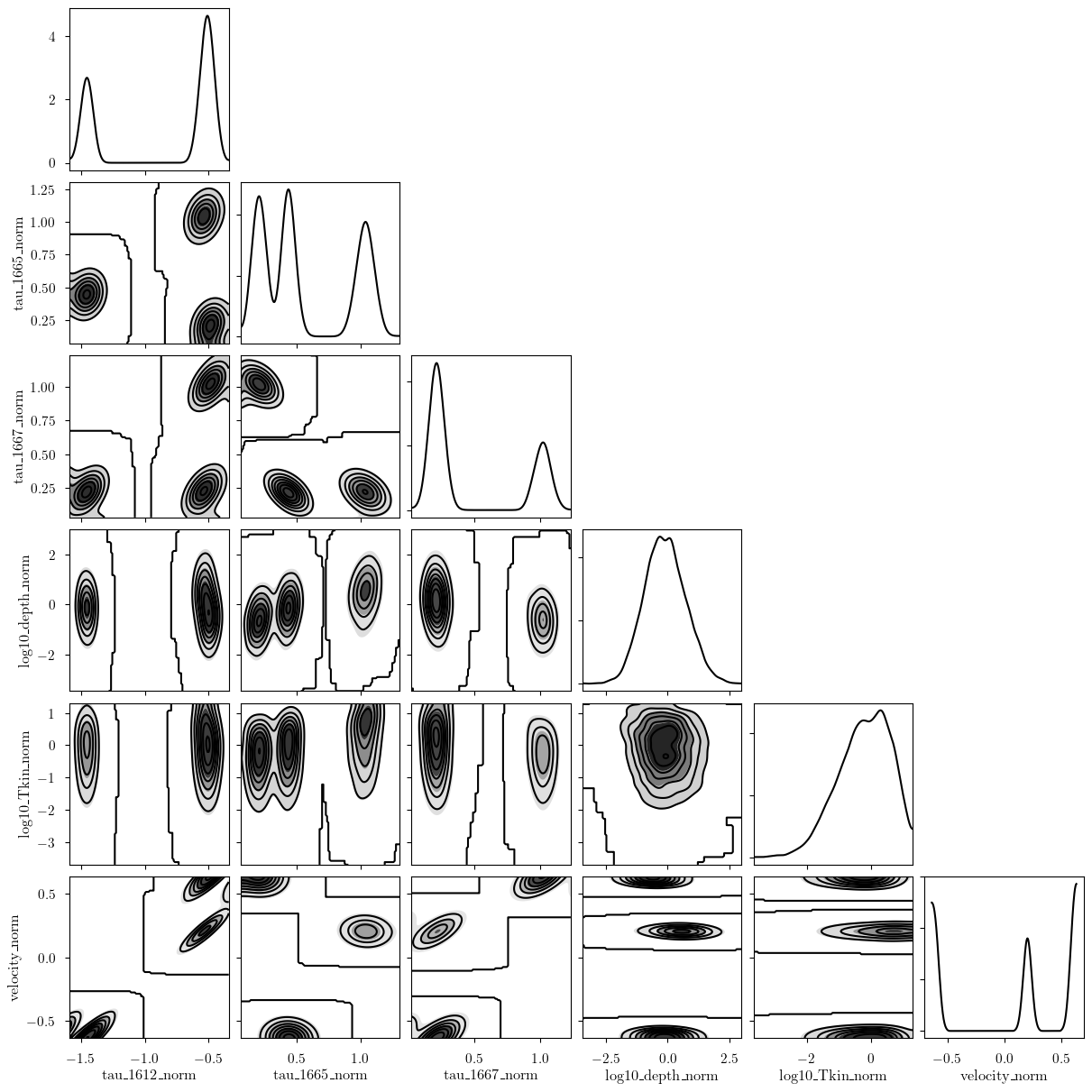
Notice that there are three posterior modes. These correspond to the three clouds of the model. We can plot the posterior distributions of the deterministic quantities for a single cloud.

var_names = ["tau_1612", "tau_1665", "tau_1667", "log10_depth", "log10_Tkin", "fwhm_nonthermal"]
axes = plot_pair(
    model.trace.solution_0.sel(cloud=0), # samples
    var_names, # var_names to plot
    labeller=model.labeller, # label manager
)
axes.ravel()[0].figure.set_size_inches(20, 20)

Finally, we can get the posterior statistics, Bayesian Information Criterion (BIC), etc.

point_stats = az.summary(model.trace.solution_0, kind='stats', stat_focus="median")
print("BIC:", model.bic())
display(point_stats)

"""
tau_params = {
    "tau_1612": np.array([-0.05, 0.05, 0.05]),
    "tau_1665": np.array([0.05, 0.1, 0.02]),
    "tau_1667": np.array([0.02, 0.02, 0.1]),
}
sim_params = {
    "log10_depth": np.array([0.0, 0.25, -0.25]),
    "log10_Tkin": np.array([1.25, 1.75, 1.0]),
    "velocity": np.array([-3.0, 1.0, 3.0]),
    "log10_nth_fwhm_1pc": 0.2,
    "depth_nth_fwhm_power": 0.3,
}
"""

BIC: -11239.35142446794

	median	mad	eti_3%	eti_97%
baseline_absorption_1612_norm[0]	-0.093	0.028	-0.168	-0.010
baseline_absorption_1665_norm[0]	-0.311	0.024	-0.377	-0.245
baseline_absorption_1667_norm[0]	-0.250	0.022	-0.315	-0.183
baseline_absorption_1720_norm[0]	0.009	0.024	-0.059	0.076
tau_1612_norm[0]	-0.537	0.027	-0.609	-0.464
tau_1612_norm[1]	-1.455	0.024	-1.523	-1.393
tau_1612_norm[2]	-0.488	0.024	-0.548	-0.418
log10_depth_norm[0]	0.512	0.484	-1.179	1.868
log10_depth_norm[1]	-0.158	0.433	-1.464	1.045
log10_depth_norm[2]	-0.638	0.414	-1.842	0.470
log10_Tkin_norm[0]	0.257	0.585	-1.636	1.182
log10_Tkin_norm[1]	-0.214	0.559	-1.960	0.815
log10_Tkin_norm[2]	-0.361	0.500	-1.964	0.637
velocity_norm[0]	0.205	0.007	0.187	0.224
velocity_norm[1]	-0.606	0.006	-0.623	-0.591
velocity_norm[2]	0.611	0.004	0.600	0.621
log10_nth_fwhm_1pc_norm	-0.407	0.378	-1.710	0.640
depth_nth_fwhm_power_norm	-0.142	0.692	-1.967	1.742
tau_1665_norm[0]	1.038	0.043	0.915	1.156
tau_1665_norm[1]	0.441	0.031	0.358	0.533
tau_1665_norm[2]	0.211	0.034	0.124	0.303
tau_1667_norm[0]	0.222	0.037	0.114	0.320
tau_1667_norm[1]	0.216	0.031	0.136	0.305
tau_1667_norm[2]	1.017	0.037	0.915	1.123
tau_1612[0]	0.046	0.003	0.039	0.054
tau_1612[1]	-0.046	0.002	-0.052	-0.039
tau_1612[2]	0.051	0.002	0.045	0.058
tau_1665[0]	0.104	0.004	0.092	0.116
tau_1665[1]	0.044	0.003	0.036	0.053
tau_1665[2]	0.021	0.003	0.012	0.030
tau_1667[0]	0.022	0.004	0.011	0.032
tau_1667[1]	0.022	0.003	0.014	0.031
tau_1667[2]	0.102	0.004	0.091	0.112
tau_1720[0]	-0.023	0.002	-0.030	-0.017
tau_1720[1]	0.057	0.003	0.050	0.064
tau_1720[2]	-0.036	0.002	-0.042	-0.030
log10_depth[0]	0.128	0.121	-0.295	0.467
log10_depth[1]	-0.040	0.108	-0.366	0.261
log10_depth[2]	-0.159	0.103	-0.461	0.117
log10_Tkin[0]	2.257	0.585	0.364	3.182
log10_Tkin[1]	1.786	0.559	0.040	2.815
log10_Tkin[2]	1.639	0.500	0.036	2.637
velocity[0]	1.025	0.034	0.936	1.120
velocity[1]	-3.032	0.030	-3.114	-2.955
velocity[2]	3.055	0.019	3.000	3.106
log10_nth_fwhm_1pc	0.159	0.038	0.029	0.264
depth_nth_fwhm_power	0.386	0.069	0.203	0.574
fwhm_thermal[0]	0.564	0.362	0.064	1.636
fwhm_thermal[1]	0.328	0.198	0.044	1.073
fwhm_thermal[2]	0.277	0.150	0.044	0.873
fwhm_nonthermal[0]	1.659	0.146	0.930	1.972
fwhm_nonthermal[1]	1.404	0.090	1.040	1.637
fwhm_nonthermal[2]	1.268	0.064	0.936	1.428
fwhm[0]	1.807	0.084	1.597	2.061
fwhm[1]	1.477	0.071	1.291	1.681
fwhm[2]	1.317	0.050	1.185	1.458

'\ntau_params = {\n    "tau_1612": np.array([-0.05, 0.05, 0.05]),\n    "tau_1665": np.array([0.05, 0.1, 0.02]),\n    "tau_1667": np.array([0.02, 0.02, 0.1]),\n}\nsim_params = {\n    "log10_depth": np.array([0.0, 0.25, -0.25]),\n    "log10_Tkin": np.array([1.25, 1.75, 1.0]),\n    "velocity": np.array([-3.0, 1.0, 3.0]),\n    "log10_nth_fwhm_1pc": 0.2,\n    "depth_nth_fwhm_power": 0.3,\n}\n'

Visualization using Mean Point Estimate

Here we demonstrate how to visualize the contribution of individual cloud components on the data from the mean posterior point estimates. Inspecting predict_tau in the model definition reveals how this works. Note that the mean posterior point estimate might not always be located within the posterior distribution (especially if there are strong parameter correlations)!

# extract parameter mean point estimates
mean_point = model.trace.solution_0.mean(dim=["chain", "draw"])
mean_point

<xarray.Dataset> Size: 480B
Dimensions:                        (baseline_coeff: 1, cloud: 3)
Coordinates:
  * baseline_coeff                 (baseline_coeff) int64 8B 0
  * cloud                          (cloud) int64 24B 0 1 2
Data variables: (12/24)
    baseline_absorption_1612_norm  (baseline_coeff) float64 8B -0.09223
    baseline_absorption_1665_norm  (baseline_coeff) float64 8B -0.3111
    baseline_absorption_1667_norm  (baseline_coeff) float64 8B -0.2504
    baseline_absorption_1720_norm  (baseline_coeff) float64 8B 0.009297
    tau_1612_norm                  (cloud) float64 24B -0.5374 -1.456 -0.4864
    log10_depth_norm               (cloud) float64 24B 0.4783 -0.1653 -0.6478
    ...                             ...
    velocity                       (cloud) float64 24B 1.026 -3.033 3.055
    log10_nth_fwhm_1pc             float64 8B 0.1551
    depth_nth_fwhm_power           float64 8B 0.3865
    fwhm_thermal                   (cloud) float64 24B 0.6637 0.4094 0.3356
    fwhm_nonthermal                (cloud) float64 24B 1.602 1.387 1.249
    fwhm                           (cloud) float64 24B 1.813 1.481 1.318

xarray.Dataset

• Dimensions:
  • baseline_coeff: 1
  • cloud: 3
• Coordinates: (2)
  • baseline_coeff
    (baseline_coeff)
    int64
    0

    array([0])

  • cloud
    (cloud)
    int64
    0 1 2

    array([0, 1, 2])

• Data variables: (24)
  • baseline_absorption_1612_norm
    (baseline_coeff)
    float64
    -0.09223

    array([-0.09222575])

  • baseline_absorption_1665_norm
    (baseline_coeff)
    float64
    -0.3111

    array([-0.3110607])

  • baseline_absorption_1667_norm
    (baseline_coeff)
    float64
    -0.2504

    array([-0.25043111])

  • baseline_absorption_1720_norm
    (baseline_coeff)
    float64
    0.009297

    array([0.00929656])

  • tau_1612_norm
    (cloud)
    float64
    -0.5374 -1.456 -0.4864

    array([-0.53736367, -1.45574568, -0.48642616])

  • log10_depth_norm
    (cloud)
    float64
    0.4783 -0.1653 -0.6478

    array([ 0.47834926, -0.16525114, -0.64777748])

  • log10_Tkin_norm
    (cloud)
    float64
    0.09615 -0.3048 -0.4431

    array([ 0.0961516 , -0.30483442, -0.4430614 ])

  • velocity_norm
    (cloud)
    float64
    0.2052 -0.6066 0.6109

    array([ 0.20521597, -0.60655114,  0.61091252])

  • log10_nth_fwhm_1pc_norm
    ()
    float64
    -0.4486

    array(-0.44857982)

  • depth_nth_fwhm_power_norm
    ()
    float64
    -0.1353

    array(-0.13531386)

  • tau_1665_norm
    (cloud)
    float64
    1.038 0.441 0.2116

    array([1.03757479, 0.44100478, 0.21158903])

  • tau_1667_norm
    (cloud)
    float64
    0.2214 0.2168 1.016

    array([0.22136218, 0.21677425, 1.01586594])

  • tau_1612
    (cloud)
    float64
    0.04626 -0.04557 0.05136

    array([ 0.04626363, -0.04557457,  0.05135738])

  • tau_1665
    (cloud)
    float64
    0.1038 0.0441 0.02116

    array([0.10375748, 0.04410048, 0.0211589 ])

  • tau_1667
    (cloud)
    float64
    0.02214 0.02168 0.1016

    array([0.02213622, 0.02167743, 0.10158659])

  • tau_1720
    (cloud)
    float64
    -0.02305 0.0568 -0.03584

    array([-0.02305256,  0.05680327, -0.0358382 ])

  • log10_depth
    (cloud)
    float64
    0.1196 -0.04131 -0.1619

    array([ 0.11958732, -0.04131278, -0.16194437])

  • log10_Tkin
    (cloud)
    float64
    2.096 1.695 1.557

    array([2.0961516 , 1.69516558, 1.5569386 ])

  • velocity
    (cloud)
    float64
    1.026 -3.033 3.055

    array([ 1.02607983, -3.03275572,  3.05456262])

  • log10_nth_fwhm_1pc
    ()
    float64
    0.1551

    array(0.15514202)

  • depth_nth_fwhm_power
    ()
    float64
    0.3865

    array(0.38646861)

  • fwhm_thermal
    (cloud)
    float64
    0.6637 0.4094 0.3356

    array([0.66365608, 0.4093964 , 0.33563565])

  • fwhm_nonthermal
    (cloud)
    float64
    1.602 1.387 1.249

    array([1.6021847 , 1.38686936, 1.24899499])

  • fwhm
    (cloud)
    float64
    1.813 1.481 1.318

    array([1.81254056, 1.48115333, 1.31771275])

• Indexes: (2)
  • baseline_coeff
    PandasIndex

    PandasIndex(Index([0], dtype='int64', name='baseline_coeff'))

  • cloud
    PandasIndex

    PandasIndex(Index([0, 1, 2], dtype='int64', name='cloud'))

• Attributes: (0)

from amoeba2 import physics

# evaluate line profile
line_profile = {}
for label in model.model.coords["transition"]:
    line_profile[label] = physics.calc_line_profile(
        model.data[f"absorption_{label}"].spectral,
        mean_point["velocity"].data,
        mean_point["fwhm"].data,
    ).eval()

# shape: spectral, clouds
print(line_profile["1612"].shape)

(400, 3)

# evaluate optical depth
tau = {}
for i, label in enumerate(model.model.coords["transition"]):
    tau[label] = mean_point[f"tau_{label}"].data * line_profile[label]

# shape: spectral, clouds
print(tau["1612"].shape)

(400, 3)

# evaluate un-normalized baseline
baseline = {}
for i, label in enumerate(model.model.coords["transition"]):
    baseline_norm = np.sum([
        mean_point[f"baseline_absorption_{label}_norm"].data[j] / (j + 1.0)**j
        * model.data[f"absorption_{label}"].spectral_norm**j
        for j in range(model.baseline_degree + 1)
    ], axis=0)
    baseline[label] = model.data[f"absorption_{label}"].unnormalize_brightness(baseline_norm)

# shape: spectral
print(baseline['1612'].shape)

(400,)

# Plot cloud contributions over data
fig, axes = plt.subplots(4, sharex=True, layout="constrained", figsize=(8, 8))
for i, label in enumerate(model.model.coords["transition"]):
    axes[i].plot(model.data[f"absorption_{label}"].spectral, model.data[f"absorption_{label}"].brightness, "k-")
    for j in range(n_clouds):
        axes[i].plot(model.data[f"absorption_{label}"].spectral, 1.0 - np.exp(-tau[label][:, j]) + baseline[label], 'r-')
    # baseline
    axes[i].plot(model.data[f"absorption_{label}"].spectral, baseline[label], 'b-')
    axes[i].set_ylabel(datum.ylabel)
_ = axes[-1].set_xlabel(datum.xlabel)